Introduction
The goal of this assignment was to create a method to determine the outline of a speed reduction zone and its effect on the local marine traffic for Dominica. The speed reduction zone encompasses the preferred habitat of the local sperm whales. This area was approximated as areas of frequent whale sightings off the coast.
# libraries for the assignment:
import pandas as pd
import geopandas as gpd
import matplotlib.pyplot as plt
import numpy as np
from shapely.geometry import Polygon
Dominica outline
We downloaded the country outline into the notebook.
fp = "data/dominica/dma_admn_adm0_py_s1_dominode_v2.shp"

dom_outline = gpd.read_file(fp)

dom_outline = dom_outline.to_crs("EPSG:4602")
We plot the outline for exploration.
fig, ax = plt.subplots(figsize=(3, 3), dpi = 200)
ax.grid(True)
dom_outline.plot(ax = ax,
                 color = "darkgreen")

ax.set_title("Dominica Outline")
ax.set_xlabel("Longitude")
ax.set_ylabel("Latitude")
Text(94.618846252753, 0.5, 'Latitude')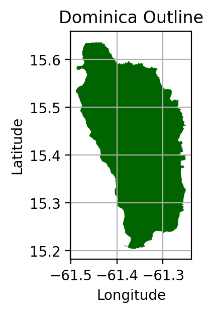
Whale sighting data
First, we read in the data and projected it into an appropriate CRS.
fp_whales = "data/sightings2005_2018.csv"

whales = gpd.read_file(fp_whales)

geometry = gpd.points_from_xy(whales.Long, whales.Lat, crs = "EPSG:4326")
whales_geom = whales.set_geometry(geometry)
Next we convert the geometries from degrees to meters.
whales_geom = whales_geom.to_crs("EPSG:2002")

dom_outline = dom_outline.to_crs("EPSG:2002")
Create a sampling grid
Making the point observations into a habitat region.
xmin, ymin, xmax, ymax = whales_geom.total_bounds

length = 2000
wide = 2000

cols = list(np.arange(xmin, xmax + wide, wide))
rows = list(np.arange(ymin, ymax + length, length))

polygons = []
for x in cols[:-1]:
    for y in rows[:-1]:
        polygons.append(Polygon([(x,y), (x+wide, y), (x+wide, y+length), (x, y+length)]))

grid = gpd.GeoDataFrame({'geometry':polygons})
grid.to_file("grid.shp")
fp_grid = "grid.shp"
grid = gpd.read_file(fp_grid)
grid = grid.set_crs("EPSG:2002")
grid = grid.to_crs("EPSG:2002")Plotting the grid to make sure it looks how we expected.
fig, ax = plt.subplots(figsize=(4, 4), dpi=200)
ax.grid(True)

grid.plot(ax = ax,
          facecolor = "none",
          lw = 0.1)
<AxesSubplot:>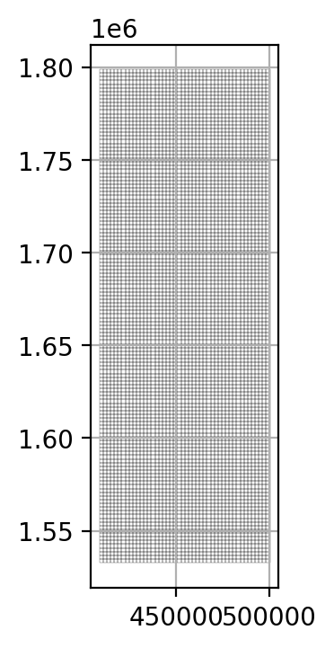
Extract the whale habitat
Now we spatially joined the grid we made in the previous step with our sighting data to count the number of sightings in each cell.
grid_join = grid.sjoin(whales_geom, how = "inner")grid['count'] = grid_join.groupby(grid_join.index).count()['index_right']grid = grid.loc[(grid['count'] > 20)]Create a convex hull
We used unary_union to create a Multipolygon containing
the union of all geometries in the GeoSeries
speed_zone = grid.unary_union
speed_zone
speed_zone = gpd.GeoSeries(speed_zone)
speed_zone = speed_zone.convex_hull
speed_zone.plot()
<AxesSubplot:>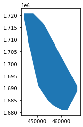
The plot above is now our habitat zone. Next we added it to the Dominica outline.
speed_zone = gpd.GeoDataFrame({'geometry':speed_zone}, crs = 2002)fig, ax = plt.subplots(figsize = (10,10), dpi = 200)
dom_outline.plot(ax = ax,
color = "darkgreen")
speed_zone.plot(ax = ax,
color = "lightyellow",
edgecolor = "black",
alpha = 0.5)
ax.set_title("Dominica Outline and Sperm Whale Habitat")
ax.set_xlabel("Longitude")
ax.set_ylabel("Latitude")Text(364.48357887628714, 0.5, 'Latitude')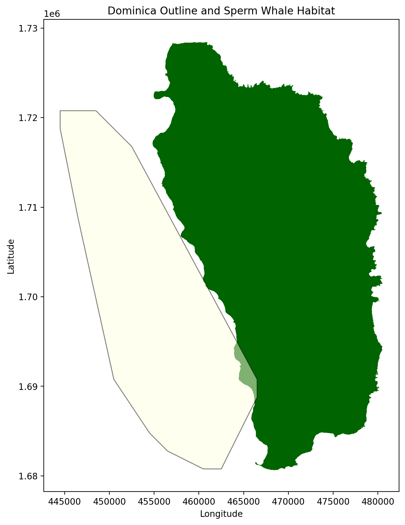
There is some overlap from the outline of Dominica and the habitat but that is fine for our calculations. Next we will upload the vessel data.
Vessel Data
Using the Automatic Identification System (AIS) we loaded the vessel data.
fp_vessels = "data/station1249.csv"

vessels = gpd.read_file(fp_vessels)

geometry = gpd.points_from_xy(vessels.LON, vessels.LAT, crs = "EPSG:4326")
vessels_geom = vessels.set_geometry(geometry)
vessels_geom = vessels_geom.to_crs("EPSG:2002")Next we explored the datatypes to make sure they are what we expected.
print(vessels_geom.dtypes)field_1 object
MMSI object
LON object
LAT object
TIMESTAMP object
geometry geometry
dtype: objectThe ‘TIMESTAMP’ data is not in datetime formatting so we changed it.
vessels_geom['TIMESTAMP'] = pd.to_datetime(vessels_geom['TIMESTAMP'], format = '%Y-%m-%d %H:%M:%S')print(vessels_geom.dtypes)field_1 object
MMSI object
LON object
LAT object
TIMESTAMP datetime64[ns]
geometry geometry
dtype: objectSetting up to calcute speed and distance
A few things needed to be done to make the necessary calculations: 1) Spatially subset vessel tracks within whale habitat 2) Sort the dataframe by MMSI and TIMESTAMP 3) Create a copy of the dataframe and shift each observation down one row using shift() and then join with the original dataset 4) Drop all rows in the joined dataframe in which the MMSI of the left is not the same as the one on the right. 5) Set the geometry column with the set_geometry() function
# 1) spatial subsetting
vessels_geom = vessels_geom.sjoin(speed_zone, how = "inner")
# 2) sorted the df by MMSI and TIMESTAMP
vessels_geom = vessels_geom.sort_values(by = ["MMSI", "TIMESTAMP"])# 3) created a copy of our df and shifted down a row then joined back with original dataset
vs_geom_copy = vessels_geom.shift(1)
# joined back with original dataset
vessels_joined = vs_geom_copy.join(vessels_geom,
how = "left",
lsuffix = 'start',
rsuffix = 'end')# 4) Dropped rows where the MMSI did not match
vessels_joined_filt = vessels_joined[vessels_joined["MMSIstart"] == vessels_joined["MMSIend"]]# 5) Set the geometry column
vessels_joined_filt = vessels_joined_filt.set_geometry("geometrystart")Calculations
- The distance for each observation to the next
- The time difference between each observation to the next
- The average speed between each observation to the next
- The time that the distance would have taken at 10 knots.
- The difference between the time that it actually took and how much it would have taken at 10 knots.
- Finally, sum up the extra time the 10 knots zone would have taken for all ships!
# 1) Distance between observations
vessels_joined_filt['distance'] = vessels_joined_filt['geometrystart'].distance(vessels_joined_filt['geometryend'])
# 2) Time difference between observations
vessels_joined_filt['time_diff'] = vessels_joined_filt['TIMESTAMPend'] - vessels_joined_filt['TIMESTAMPstart']# 3) The average speed between each observation
vessels_joined_filt['avg_speed_m_s'] = vessels_joined_filt['distance']/vessels_joined_filt['time_diff'].dt.total_seconds()# 4) Time that the distance would have taken at 10 knots.
# 10 knot = 5.1444 m/s
kts_10 = 5.1444
vessels_joined_filt['time_10kts_tot_s'] = (vessels_joined_filt['distance'] / kts_10)# 5) Difference between the time that it actually took and time it would have taken at 10 knots
vessels_joined_filt['time_10kts_diff_hr'] = (vessels_joined_filt['time_10kts_tot_s'] - vessels_joined_filt['time_diff'].dt.total_seconds()) / (60 *60)
# Below is what the head() of the data looks like after adding the columns from these calculations
vessels_joined_filt.head()| field_1start | MMSIstart | LONstart | LATstart | TIMESTAMPstart | geometrystart | index_rightstart | field_1end | MMSIend | LONend | LATend | TIMESTAMPend | geometryend | index_rightend | distance | time_diff | avg_speed_m_s | time_10kts_tot_s | time_10kts_diff_hr | |
|---|---|---|---|---|---|---|---|---|---|---|---|---|---|---|---|---|---|---|---|
| 235018 | 235025 | 203106200 | -61.40929 | 15.21021 | 2015-02-25 15:32:20 | POINT (462476.396 1680935.224) | 0.0 | 235018 | 203106200 | -61.41107 | 15.21436 | 2015-02-25 15:34:50 | POINT (462283.995 1681393.698) | 0 | 497.209041 | 0 days 00:02:30 | 3.314727 | 96.650541 | -0.014819 |
| 235000 | 235018 | 203106200 | -61.41107 | 15.21436 | 2015-02-25 15:34:50 | POINT (462283.995 1681393.698) | 0.0 | 235000 | 203106200 | -61.41427 | 15.22638 | 2015-02-25 15:42:19 | POINT (461936.769 1682722.187) | 0 | 1373.116137 | 0 days 00:07:29 | 3.058165 | 266.914730 | -0.050579 |
| 234989 | 235000 | 203106200 | -61.41427 | 15.22638 | 2015-02-25 15:42:19 | POINT (461936.769 1682722.187) | 0.0 | 234989 | 203106200 | -61.41553 | 15.2353 | 2015-02-25 15:47:19 | POINT (461798.818 1683708.377) | 0 | 995.792381 | 0 days 00:05:00 | 3.319308 | 193.568226 | -0.029564 |
| 234984 | 234989 | 203106200 | -61.41553 | 15.2353 | 2015-02-25 15:47:19 | POINT (461798.818 1683708.377) | 0.0 | 234984 | 203106200 | -61.41687 | 15.23792 | 2015-02-25 15:49:50 | POINT (461654.150 1683997.765) | 0 | 323.533223 | 0 days 00:02:31 | 2.142604 | 62.890371 | -0.024475 |
| 234972 | 234984 | 203106200 | -61.41687 | 15.23792 | 2015-02-25 15:49:50 | POINT (461654.150 1683997.765) | 0.0 | 234972 | 203106200 | -61.41851 | 15.24147 | 2015-02-25 15:54:49 | POINT (461476.997 1684389.925) | 0 | 430.317090 | 0 days 00:04:59 | 1.439188 | 83.647673 | -0.059820 |
# 6) Final calculation
increased_time = vessels_joined_filt[vessels_joined_filt['time_10kts_diff_hr'] > 0]
print("The increased travel time for the ship traffic is ",
      round((increased_time['time_10kts_diff_hr'].sum())/24, 2),
     " days.")
The increased travel time for the ship traffic is 27.88 days.